Modeling Disordered Quantum Systems: Random Edge Laplacians
This is joint work done with my advisor Günter Stolz.
The following video shows the level statistics of the eigenvalues of a random operator. Read on for a full explanation of what can be seen.
The most important object in the quantum mechanical description of physical systems is the Hamiltonian \(H\). In mathematical terms, the Hamiltonian is a self-adjoint operator in a Hilbert space. The spectrum of \(H\) gives the possible energies which the physical system can have, while the eigenfunctions of \(H\) correspond to the states of the system. Moreover, the solution of the time-dependent Schrödinger equation \[ H \psi(t) = i\frac{d}{dt} \psi(t), \quad \psi(0) = \psi_0 \] describes the physical time-evolution of a system with initial state \(\psi_0\). Determining the spectrum, eigenfunctions, and time-evolution of a self-adjoint operator requires deep tools from functional analysis, operator theory, as well as spectral and scattering theory. Due to their applications in quantum mechanics, these areas of mathematics play important roles in theoretical physics and continue to be very active research fields.
The explicit form of the Hamiltonian depends on the physical system it describes. For example, the Hamiltonian describing an (idealized) one-dimensional electron moving in a conservative force field generated by the potential function \(V:\mathbb{R} \to \mathbb{R}\) is given by \[ H \psi = -\psi'' + V \psi.\] It acts on sufficiently smooth functions \(\psi\) (i.e. functions which can be twice differentiated) in the Hilbert space \[ L^2(\mathbb{R}) = \left\{ \psi:\mathbb{R} \to \mathbb{C}: \int_{\mathbb{R}} |\psi(x)|^2\,dx \lt \infty \right\}.\]
In theoretical physics and, in particular, in condensed matter physics, discretized versions of the above Hilbert space and Hamiltonian are frequently used. In this setting \(\mathbb{R}\) is replaced by the lattice \(\mathbb{Z}\) and the Hilbert space becomes the space of square-summable doubly infinite sequences \[ \ell^2(\mathbb{Z}) = \left\{ \varphi =(\ldots , \varphi_{-1}, \varphi_0,\varphi_1,\ldots) : \sum_{j=-\infty}^\infty |\varphi_j|^2 \lt \infty \right\}.\] A discrete potential is a function \(V:\mathbb{Z} \to \mathbb{R}\) and the discretized version \(h\) of the Hamiltonian \(H\) is acting on \(\varphi \in \ell^2(\mathbb{Z})\) as \begin{equation} \label{discSO} (h\varphi)(n) = - \varphi(n-1) +2\varphi(n) - \varphi(n+1) + V(n) \varphi(n). \end{equation} The term \(2\varphi(n)\) on the right is frequently suppressed because it is mathematically and physically trivial (it corresponds to a constant energy shift by 2), but it is useful for us to include it in the definition of \(h\).
Physical systems are often disordered. For example, physical materials such as crystals often have impurities (an example being given by diamonds). Electrons moving in such materials will be exposed to random forces. The Hamiltonians of such systems are modeled by random operators, with the historically first and most studied example given by the Anderson model. This model takes the form \(\eqref{discSO}\) with the values of the potential \(V(n)\), \(n\in \mathbb{Z}\), given by a sequence of independent, identically distributed (i.i.d.) random variables. One might say that the potential is generated by an infinite number of coin tosses.
While the Anderson model is the best understood example of a random operator, there are other models of random operators which are physically relevant and mathematically interesting (as well as challenging). Reaching a better understanding of one such model, the so-called random edge Laplacian, is the goal of our work. Below we introduce the one-dimensional version of this model, describe some of its known properties, and state some open problems and conjectures, which we motivate by numerical investigations.
The underlying Hilbert space for this model is again \(\ell^2(\mathbb{Z})\). We will use the notation that for \(\phi \in \ell^2(\mathbb{Z})\) such that \(\Vert \phi \Vert =1\), \(P_\phi = |\phi\rangle \langle \phi |\) is the orthogonal projection onto \(\phi\). Also, we define \[ \alpha_n := \frac{1}{\sqrt{2}}(\delta_n - \delta_{n+1}).\] We will call these vectors "edge vectors."
We can now define a function \(b: \{ \{n,n+1\}: n\in \mathbb{Z} \} \to (0,\infty)\), which we think of as assigning a positive, finite weight to each of the edges connecting neighboring points of the graph with vertices \(n\in \mathbb{Z}\). We will use the shorthand \(b_n := b(\{n,n+1\})\). Our weights \(b=(b_n)_{n \in \mathbb{Z}}\) can now be assigned as i.i.d. random variables. We assume that their common distribution measure \(\mu\) is absolutely continuous and such that \(\rm{supp}\, \mu = [c_1,c_2]\) with \(0 \lt c_1 \lt c_2 \lt \infty\).
We define a random operator on \(\ell^2(\mathbb{Z})\) as: \[ (L_b \varphi)(n) = -b_{n-1} \varphi(n-1) + (b_{n-1} + b_n)\varphi(n) - b_n \varphi (n+1) . \] Comparing with \(\eqref{discSO}\), we see that \(L_b\) does not include a random potential, but now each term includes a random weight. It becomes convenient to think of \(b_n\) as a weight on the edge connecting vertices \(n\) and \(n+1\). Thus leading us to refer to \(L_b\) as a random edge Laplacian.
Other ways of representing \(L_b\) are via its quadratic form \[ \langle \varphi,L_b\varphi \rangle = \sum_{n \in \mathbb{Z}} b_n \vert \varphi(n+1)-\varphi(n)\vert^2. \] or as a sum of projections \[ L_b = 2\sum_{n \in \mathbb{Z}} b_n P_{\alpha_n} .\] In particular, \(L_b \geq 0\). Also, it can be shown that \(\sigma(L_b) = [0,4c_2]\) almost surely. Using the canonical basis for \(\ell^2(\mathbb{Z})\), we can write \(L_b\) as the infinite matrix \[ L_b = \begin{pmatrix} \ddots&\ddots&\ddots&&&& \\ &-b_{-2}&b_{-2}+b_{-1}&-b_{-1}&&& \\ &&-b_{-1}&b_{-1}+b_0&-b_0&& \\ &&&-b_0&b_0+b_1&-b_1& \\ &&&&\ddots&\ddots&\ddots \end{pmatrix}. \]
The following numerical analysis of \(L_b\) was done through the use of MATLAB and Octave. These results were done with the common distribution \(\mu\) for the edges being the uniform distribution on \([1,2]\). We begin by introducing a few definitions.
For a given \(E \in \mathbb{C}\), the \(n\)-th transfer matrix for \(L_b\) is given by
\[ \tilde{A}(E,n):= \begin{pmatrix}0&1\\ -\frac{b_{n-1}}{b_n} & \frac{b_{n-1}+b_n-E}{b_n}\end{pmatrix}.\]
These are called transfer matrices because \(\varphi\) solves \((L_b-EI)\varphi =0\) if and only if
\[ \begin{pmatrix}\varphi(n) \\ \varphi(n+1)\end{pmatrix} = \tilde{A}(E,n) \begin{pmatrix}\varphi(n-1) \\ \varphi(n)\end{pmatrix}\] for all \(n \in \mathbb{Z}\). Transfer matrices are a useful tool in studying operators. However, for our purposes, we would like the transfer matrices to be independent and have determinant one. We can easily see that these matrices do not generally have determinant one and as they depend on two random variables, they are not indepenedent. Thus, we define a new type of transfer matrix.
For a given \(E \in \mathbb{C}\), the \(n\)-th modified transfer matrix for \(L_b\) is given by
\[ A_b(n,E) := \begin{pmatrix}1&-E\\\frac{1}{b_n}&1-\frac{E}{b_n}\end{pmatrix}.\]
We are still able to think of these matrices as transfer matrices because a function \(\varphi\) solves \((L_b - EI)\varphi =0\) if and only if
\[ \begin{pmatrix} b_n ( \varphi(n+1)-\varphi(n) ) \\ \varphi(n+1) \end{pmatrix} = A_b(n,E) \begin{pmatrix} b_{n-1} ( \varphi(n)-\varphi(n-1) ) \\ \varphi(n) \end{pmatrix}. \]
Define, for \(n>0\),
\[ T_b(n,E) := A_b(n,E)\cdots A_b(1,E).\]
Then, for a solution \(\varphi\) of \((L_b-EI)\varphi=0\), we have
\[ \begin{pmatrix} b_n(\varphi(n+1)-\varphi(n)) \\ \varphi(n+1) \end{pmatrix} = T_b(n,E) \begin{pmatrix} b_0 (\varphi(1)-\varphi(0)) \\ \varphi(1) \end{pmatrix}.\]
We then define the following value.
For \(E \in \mathbb{C}\), the quantity
\[ \gamma(E) := \lim_{n\to \infty} \mathbb{E} \left( \frac1n \ln \Vert T_{(\cdot )} (n,E) \Vert \right) \]
is called the Lyapunov exponent. Here \(\mathbb{E}(\cdot)\) denotes averaging over the random variables \(b_n\).
It can be shown that Lyapunov exponents are non-negative and that \(\gamma(E)\) does not change if we use our standard transfer matrices or our modified transfer matrices. When looking at the Lyapunov exponent, we are interested in knowing for what values of \(E\), \(\gamma(E)\) is positive. In order to get an idea of what to expect, we have plotted the Lyapunov exponent for the \(600 \times 600\) approximation of \(L_b\).
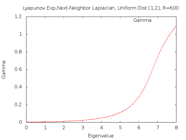
The graph suggests that the Lyapunov exponent is positive away from zero, but we would like a closer look at what happens as \(E\) goes to zero. The following graph is a magnification of the previous graph around zero.
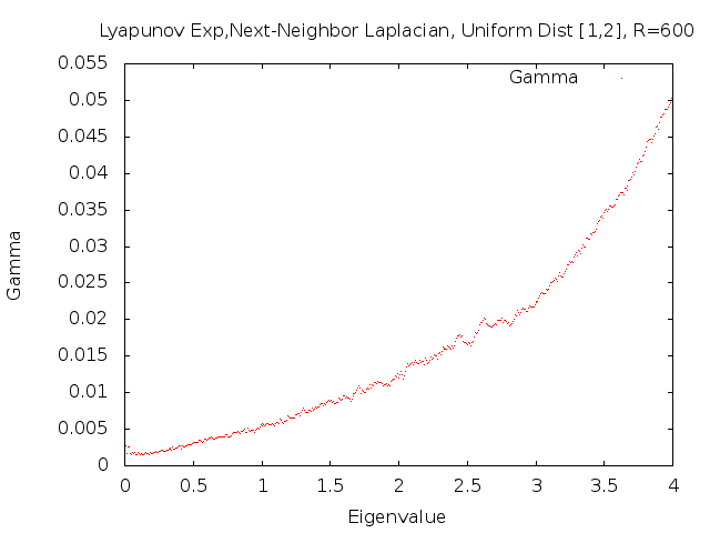
We are now reasonably sure that the Lyapunov exponent is positive for non-zero \(E\), but we can't be sure what happens for \(E=0\). This is where our numerical approach ends and we turn to analytical methods.
We can show via Fürstenberg's Theorem that \(\gamma(E)>0\) for \(E>0\). We can also show, through direct calculation using the modified transfer matrices, that \(\gamma(0)=0\). This is an important difference between this model and the Anderson model, where it is known that Lyapunov exponents are positive for all values of \(E\). Our next goal will be to determine how \(\gamma\) goes to zero as \(E\) goes to zero. In particular, we would like to show that the convergence is linear.
The next property of \(L_b\) that we will investigate is the density of states. In order to define the density of states we first define the integrated density of states.
Let \(L_{b,N}\) be the restriction of \(L_b\) to the box \([-N,N]\). Then the integrated density of states of \(L_b\) is given almost surely by
\[ \mathcal{N}(E) := \lim_{N\to \infty} \frac{1}{2N+1} \#\{ \mbox{eigenvalues of $L_{b,N}$} \leq E \}.\]
The density of states can then be defined.
The density of states of \(L_b\) is given by
\[ n(E):= \frac{d}{dE}\mathcal{N}(E).\]
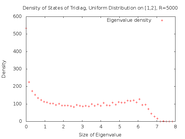
As \(\mathcal{N}(E)\) is non-decreasing in \(E\), its derivative \(n(E)\) must exist at least Lebesgue-almost everywhere.The following graph gives the density of states for the \(5000 \times 5000\) approximation of \(L_b\). As we mentioned earlier, we can show that the almost-sure spectrum of \(L_b\) is \([0,4c_2]\), where \(c_2\) is the upper bound on the support of the common distribution \(\mu\). In this case, \(c_2=2\). Thus, the almost-sure spectrum is \([0,8]\).
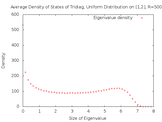
We can obtain a better graph by averaging the density of states of 100 independent trials.
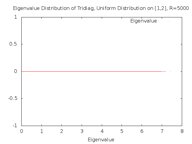
Now that we have investigated the density of the eigenvalues, we look at the actual distributions of the eigenvalues. As we mentioned earlier, the almost-sure spectrum is \([0,8]\). Thus, plotting all of the eigenvalues gives us the following graph.
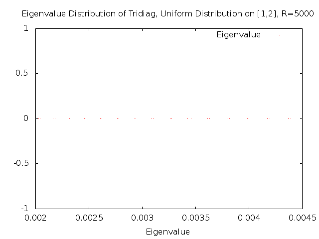
We now zoom in to look at very local pieces of the spectrum. As you can see in the next graph, very close to zero the eigenvalues appear to come in pairs. Furthermore, those pairs of eigenvalues appear to be regularly spaced from the other pairs.
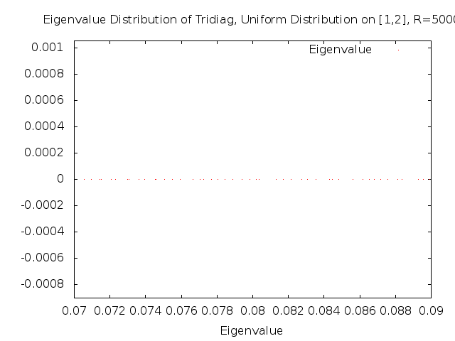
Continuing along the spectrum we can see that the pair structure which we saw before is now gone, but it isn't clear that the distribution of the eigenvalues has become random.
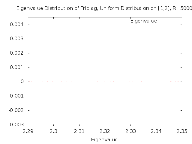
Further along the spectrum, the distribution of the eigenvalues appears to have become random.
In order to see more clearly when the distribution of eigenvalues is regular or random, we look at the distribution of the distances between the eigenvalues. Since we expect the distribution to change over the course of the spectrum, we will look at small batches of eigenvalues and move through the spectrum. In order the do this, the eigenvalues of a \(20000 \times 20000\) approximation of \(L_b\) were sorted least to greatest. After that, the first 150 eigenvalues were taken and the distances between consecutive eigenvalues were calculated. These distances were normalized and a histogram was then created. This is the first frame of the video at the top of this page. For the second frame, eigenvalues 6-155 were put through the same process. This was repeated until we exhausted all of the eigenvalues.
If the eigenvalues are regularly spaced, we will see histograms which look like delta peaks. If the eigenvalues are randomly spaced, the histograms will look like exponential decays. As you can see, very early in the video we see two peaks. These peaks correspond to the paired spacing we saw earlier. These peaks then seem to merge and the distribution appears to go through a transition period before becoming exponential decay.